Kourganoff graphs

Scharzschild equation provides a tool to easily find and analyze the solution of the radiative transfer cases for some simple source functions. First of all, the lambda operator is clearly linear, so $$\begin{equation} \Lambda[a\,f(t) + b\,g(t)] = a\,\Lambda[f(t)] + b\,\Lambda[g(t)]. \end{equation}$$


(i) The operator applied to $S(\tau) = 1$ and $S(\tau) = \tau$ can be expressed by exponential integrals (for the proof see Kourganoff, 1952, pp.43-45):
$$\begin{eqnarray*} \Lambda[1] &=& 1 - \frac{1}{2}\,E_2(\tau),\\ \Lambda[t] &=& \tau + \frac{1}{2}\,E_3(\tau). \end{eqnarray*}$$
(ii) When the lambda operator is applied to the exponential function, the result is (ibid, p.46):
$$\begin{eqnarray*} \Lambda[\exp(-at)] &=& \frac{\exp(-at)}{2a}\left[\ln\frac{a+1}{|a-1|}-E_1(\tau-\tau a)\right] + \frac{1}{2a}E_1(\tau), \;\;\;\;&a& > 0, a \ne 1;\\ \Lambda[\exp(-t)] &=& \frac{1}{2}\exp(-\tau)[\ln 2\tau + \gamma] + \frac{1}{2}E_1(\tau), \;\;\;\;&a& = 1, \end{eqnarray*}$$
where $\gamma = 0.577215$ is the Euler-Mascheroni constant.
(iii) When it is applied to a pulse function ($S = 1$ between $\tau_1$ and $\tau_2$, otherwise $S = 0$).
$$\begin{eqnarray*} \Lambda[S] &=& \frac{1}{2}\left[E_2(\tau_1 - \tau) - E_2(\tau_2 - \tau)\right], \;\;\;\;&0 &\le  \tau < \tau_1;\\ \Lambda[S] &=& 1 - \frac{1}{2}\left[E_2(\tau - \tau_1) - E_2(\tau_2 - \tau)\right], \;\;\;\;&\tau_1&\le \tau < \tau_2;\\ \Lambda[S] &=& \frac{1}{2}\left[E_2(\tau - \tau_2) - E_2(\tau - \tau_1)\right], \;\;\;\;&\tau&> \tau_2. \end{eqnarray*}$$

Graphs

Kourganoff (ibid, pp.50-54) provides graphs where some elementary source functions are compared to the result of the lambda operator action on them. Here we reproduce these graphs using the IDL intrinsic functions.

Constant source function, $S = 1$

,

Linear source function, $S = 1 + a\tau$ with $\tau = \frac{1}{2}, \frac{3}{2}, 3$

Exponential source function, $S = \exp(-a \tau)$ with $a = 0.5, 1$

Pulse source function

IDL

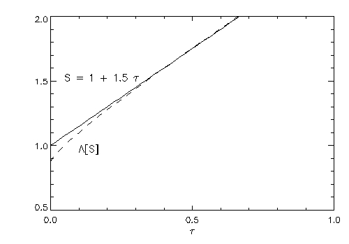
The IDL routine used to plot the graphs is kourganoff_plots.pro.

Interpratation

In radiative equilibrium, the lambda operator maps the source function to itself. If $S_\mathrm{e}$ is the exact solution, we can write:
$$\begin{equation} S_\mathrm{e} = \Lambda[S_\mathrm{e}]. \end{equation}$$
However, for some approximative solution $S_\mathrm{a} = S_\mathrm{e} + \Delta S$, we can write:
\begin{eqnarray*}
\Lambda[\Delta S] &=& \Lambda[S_\mathrm{a} - S_\mathrm{e}] = \\&=&\Lambda[S_\mathrm{a} - S_\mathrm{e}] = \\
\\&=&\Lambda[S_\mathrm{a}] - \Lambda[S_\mathrm{e}] = \\
\\&=&\Lambda[S_\mathrm{a}] - S_\mathrm{e}.
\end{eqnarray}
Thus, if the errors of the approximation with the optical depth are close to an elementary function, the Kourganoff graphs tell us how much we can hope to improve the solution at certain optical depth with one application of the lambda operator. Well, this leads us toward one of the following steps/posts - toward the lambda iteration.

Note: For the proof of the result of the lambda operator on the pulse function Kourganoff directs the reader to a paper by Unsöld (1948, Zeit. f. Astrophys, 24, 363, Über die Integralgleichung des Strahlungsgleichgewichtes in Sternatmosphaeren). However, that paper is not included (not even as a refernce) in the ADS database. So, if your interested in the proof either be ready to dig through an old library or to derive it yourself. The latter seems more doable and as a good fun for rainy days.

Note: These graphs are common in many books on the radiative transfer theory (see Rutten, 2003, p.83).