Cubic spline interpolation: Natural splines

Last year I published a post on the data interpolation and smoothing using the cubic splines using IDL. (Soon I'll do an update of that post as well.) Here I go a step back and show how the classical spline interpolation works. As before, the derivation follows the book of D.S.G.Pollock (highly recommended to any student interested in the analysis of time-series). I'll first go through some theory general for all the cubic splines, than through the derivation of the natural cubic splines and at the end I'll show some examples. In the next post I'll describe the solution of the clamped cubic splines and do the same examples using that variation of the method.

The task is to interpolate an a priori uknown function $y$ that is sampled at $n$ discrete values of the variable $x_i (i = 1, \dots, n)$ ($x_i$'s are called nodes). The values $x_i$ are assumed to be sorted in the monotonic order. The number of the segments between the $x_i$ points is $n-1$. The width of the $i$-th segment is
\begin{equation}
h_i = x_{i+1} - x_{i}.
\label{eq:h}
\end{equation}
The unknown function may be replaced piece-wise (segment-by-segment) by third-order polynomials (so-called cubic splines). In addition, the smoothness of the entire function is required, thus the continuity of the first and second derivative of the function at the nodes. The solution of the problem consists in finding the four coefficients of the 3rd-order polynomial $(a_i, b_i, c_i, d_i)$ for each segment $i = 0, \dots, n-1$.  Once they are known, it is trivial to compute the approximative function $S(x)$ for any value of $x \in [x_0, x_n]$. The function $S$ and its derivatives at the segment $i$ are:
\begin{eqnarray}
S_i(x) &=& a_i + b_i\,(x-x_i) + c_i\,(x-x_i)^2 + d_i\,(x-x_i)^3,\\
S'_i(x) &=& b_i + 2c_i\,(x-x_i) + 3d_i\,(x-x_i)^2,\\
S''_i(x) &=& 2c_i + 6d_i\,(x-x_i),\\
S^{(3)}_i(x) &=& 6d_i,\\
S^{(4)}_i(x) &=& 0.
\end{eqnarray}
The total number of the unknown coefficients is $4(n-1)$.

The equations are derived from the 3 conditions that must be fulfilled at all of the inner nodes $(i = 2, \dots, n-1)$:

(i) Continuity of the functions $S(x)$:
\begin{equation}
S_{i-1}(x_i) = S_i(x_i),\;\;\;\;\; i = 1, \dots, n-1,
\label{eq:cont0}
\end{equation}
where
$$
S_{i-1}(x) = a_{i-1} + b_{i-1}\,(x-x_{i-1}) + c_{i-1}\,(x-x_{i-1})^2 + d_{i-1}\,(x-x_{i-1})^3.
$$
and
$$
S_i(x) = a_i + b_i\,(x-x_i) + c_i\,(x-x_i)^2 + d_i\,(x-x_i)^3.
$$
At $x = x_i$ the condition in Eq.\ref{eq:cont0} reads:
$$
a_{i-1} + b_{i-1}(x_i - x_{i-1}) + c_{i-1} (x_i - x_{i-1})^2 + d_{i-1}(x_i - x_{i-1})^3 = a_{i},
$$
$$
a_{i-1} + b_{i-1} h_{i-1} + c_{i-1} h_{i-1}^2 + d_{i-1} h_{i-1} ^3 = a_i.
$$
The last equation is solved for $b_{i-1}$:
$$
b_{i-1} = \frac{a_i - a_{i-1}}{h_{i-1}} - c_{i-1}  h_{i-1} - d_{i-1} h_{i-1} ^2.
$$

Finally, from the continuity of the function it also follows that $a_i \equiv y_i$, so the number of the unknown coefficients is reduced to $3(n-1)$, thus:

\begin{equation}
b_{i-1} = \frac{y_i - y_{i-1}}{h_{i-1}} - c_{i-1}  h_{i-1} - d_{i-1} h_{i-1} ^2.
\label{eq:1st}
\end{equation}

(ii) Continuity of the first derivative:
\begin{equation}
S'_{i-1}(x_i) = S'(x_i)_i,\;\;\;\;\; i = 1, \dots, n-1
\label{eq:cont1}
\end{equation}

The continuity of the first derivative  leads in a similar way to (at $x = x_i$):

$$
b_{i-1} + 2c_{i-1} (x_i - x_{i-1}) + 3d_{i-1}(x_i - x_{i-1})^2 = b_i,
$$
or:

\begin{equation}
b_i - b_{i-1} = 2c_{i-1} h_{i-1} + 3d_{i-1} h_{i-1}^2.
\label{eq:2nd}
\end{equation}

(iii) Continuity of the second derivative:
\begin{equation}
S''_{i-1}(x_i) = S''(x_i)_i, \;\;\;\;\; i = 1, \dots, n-1.
\label{eq:cont2}
\end{equation}

The continuity of the second derivative (at $x = x_i$) can be expressed as:

$$
2c_{i-1} + 6d_{i-1}(x_i - x_{i-1})^2 = 2c_i,
$$
or:

\begin{equation}
d_{i-1}  = \frac{c_i - c_{i-1}}{3 h_{i-1}}.
\label{eq:3rd}
\end{equation}

In addition, the equations \ref{eq:1st}, \ref{eq:2nd} and \ref{eq:3rd} can be written for the next node  $x = x_{i+1}$:

\begin{equation}
b_i = \frac{a_{i+1} - a_i}{h_i} - c_i  h_i - d_i h_i ^2.
\label{eq:1st1}
\end{equation}
\begin{equation}
b_{i+1} - b_i = 2c_i h_i + 3d_i h_i^2.
\label{eq:2nd1}
\end{equation}
\begin{equation}
d_i  = \frac{c_{i+1} - c_i}{3 h_i}.
\label{eq:3rd1}
\end{equation}

Note that the Eqs. \ref{eq:1st}, \ref{eq:2nd} and \ref{eq:3rd} can be written for $i = 0, n-1$, while Eqs.\ref{eq:1st1}, \ref{eq:2nd1} and \ref{eq:3rd1} hold for $i = 1, n$. In the latter the index $n$ formally refer to a function $S_n$ that is already out of the limits of the array $x_i$. We won't explicitly compute that function, though we will use it to specify the boundary condition.

In the next step the values  of $d_i$ and $d_{i-1}$ in Eqs.\ref{eq:1st}, \ref{eq:1st1} and \ref{eq:2nd} are replaced using Eqs.\ref{eq:3rd} and \ref{eq:3rd1}.

Equations \ref{eq:1st} and \ref{eq:1st1} now become (for $i = 0, \dots, n-1$ and $i = 1, \dots, n$ respectively):
\begin{equation}
b_{i-1} =\frac{y_i - y_{i-1}}{h_{i-1}} -  \frac{(c_i + 2c_{i-1})}{3} h_{i-1},
\label{eq:1st2}
\end{equation}
\begin{equation}
b_i = \frac{y_{i+1} - y_i}{h_i} - \frac{(c_{i+1} + 2c_i) }{3} h_i.
\label{eq:1st3}
\end{equation}

The difference of Eqs.\ref{eq:1st3} and \ref{eq:1st2} equals to the right-hand side of Eq.\ref{eq:2nd1} so the $b$-coefficients are eliminated. After some simple rewritting we get:

\begin{eqnarray}
y_{i+1}\frac{3}{h_i} + y_i \left(-\frac{3}{h_i}-\frac{3}{h_{i-1}} \right) + y_{i-1}\frac{3}{h_{i-1}} = \nonumber\\ =
c_{i+1}h_i + 2c_i (h_{i-1} + h_i) + c_{i-1}h_{i-1}.
\label{eq:ac}
\end{eqnarray}

We can write $n-1$ equations like this for $i = 1, \dots, n-1$. we have $n-1$ equations for $n$ unknown coefficients $c_i$. To solve the system we still need to specify the boundary conditions at the edges of the interval for $c_1$ and $c_n$. There are two common choices:

(i) Natural splines: the second derivative of $S(x)$ at the boundaries is equal 0:
\begin{equation} S''_0(x_0) = 2c_0 = 0, \;\;\;\;\;\;\;S_{n}''(x_n) = 2c_n = 0.
\label{eq:natural}
\end{equation}    

(ii) Clamped splines: the first derivative of $S(x)$ at the boundaries is equal to the first derivative of the function $y$ in these points:
\begin{equation}
S'_0(x_0) =b_0 = y'(x_0), \;\;\;\;\;\;\;S_{n}''(x_n) = b_n = y'(x_n).
\label{eq:clamped}
\end{equation}             

The numerical implementation of the natural splines is somewhat simpler, so we start from there.

Natural splines

Let's write Eqs.\ref{eq:ac} as
\begin{equation}
q_i = c_{i-1}h_{i-1}+c_{i}w_{i} + c_{i+1}h_{i},
\label{eq:qwsystem}
\end{equation}
where
\begin{equation}
w_i = 2(h_i + h_{i-1}) = 2(x_{i+1} - x_i + x_i - x_{i-1}) = 2(x_{i+1}-x_{i-1}),
\label{eq:w}
\end{equation}
and
\begin{equation}
q_i = y_{i+1}\frac{3}{h_i} + y_i \left(-\frac{3}{h_i}-\frac{3}{h_{i-1}} \right) +y_{i-1}\frac{3}{h_{i-1}}.
\label{eq:q}
\end{equation}
There is n-1 values of q and w with the indices running from 1 to n-1. For $i = 1$:
\begin{equation} q_1 = c_0 h_0 +c_1w_1 + c_2 h_1 = c_1w_1 + c_2 h_1. \label{eq:qwsystem1} \end{equation} For $i = n-1$:
\begin{equation} q_{n-1} = c_{n-2}h_{n-2}+c_{n-1}w_{n-1} + c_{n}h_{n-1} = c_{n-2}h_{n-2}+c_{n-1}w_{n-1}. \label{eq:qwsystem2} \end{equation} The system Eq.\ref{eq:qwsystem} in the matrix form becomes:
\begin{equation}\left(\begin{matrix} q_1 \\ q_2 \\ \vdots \\ q_{n-2}  \\q_{n-1}\end{matrix}\right)=
\left(\begin{matrix} w_1 & h_1 & 0   & \dots & 0   & 0  & 0 \\
h_1 & w_2 & h_2 & \dots & 0   & 0  & 0\\
\vdots & \vdots & \vdots & \ddots & \vdots   & \vdots  & \vdots  \\
0 & 0 & 0 & \dots & h_{n-3} & w_{n-2} & h_{n-2}  \\
0 & 0 & 0 & \dots & 0 & h_{n-2} & w_{n-1} \end{matrix}\right)
\left(\begin{matrix} c_1 \\ c_2 \\ \vdots \\ c_{n-2}  \\c_{n-1}\end{matrix}\right),
\label{eq:matrix1}\end{equation}.

The system is tridiagonal, but it can be reduced to a bidiagonal using Gaussian elimination. First solve the first equation ($i = 1$) for $c_1$:
$$q_1 = w_1 c_1 + h_1 c_2 \Rightarrow c_1 = \frac{q_1}{w_1} - \frac{h_1}{w_1} c_2.$$
When that is replaced to the second equation ($i=2$), it becomes:
\begin{eqnarray} &q_2& = h_1 c_1 + w_2 c_2 + h_2 c_3, \nonumber\\
&\Rightarrow& q_2 = h_1 \left(\frac{q_1}{w_1} - \frac{h_1}{w_1} c_2\right) + w_2 c_2 + h_2 c_3,\nonumber\\
&\Rightarrow& q_2 - h_1 \frac{q_1}{w_1}= \left(w_2 - \frac{h_1^2}{w_1} \right)c_2 + h_2 c_3,\nonumber\\
&\Rightarrow& q_2' = w_2' c_2 + h_2 c_3,\nonumber \end{eqnarray}

where
$$q_2' = q_2 - h_1 \frac{q_1}{w_1} \;\;\;\;\mathrm{and}\;\;\; w_2' = w_2 - \frac{h_1^2}{w_1}.$$

Further, for any $i = 2, \dots, n-2$ we can write:
\begin{equation}
q_i = h_{i-1} c_{i-1} + w_{i} c_{i} + h_{i} c_{i+1} \Rightarrow q_i' = w_i' c_i + h_i c_{i+1},
\label{eq:qprimi}
\end{equation}
with
\begin{equation}
q_i' = q_i - h_{i-1} \frac{q_{i-1}}{w_{i-1}} \;\;\;\;\mathrm{and}\;\;\; w_i' = w_i - \frac{h_{i-1}^2}{w_{i-1}}
\label{eq:qwprim}.
\end{equation}
For $i = n-1$ the equation is directly solvable:
\begin{equation}
q_{n-1}' = w_{n-1}' c_{n-1} + h_{n-1} c_n = w_{n-1}' c_{n-1}.
\label{eq:qprimnm1}
\end{equation}

The system in Eq.\ref{eq:matrix1} now becomes bidiagonal:

\begin{equation}\left(\begin{matrix} q_1' \\ q_2' \\ \vdots \\ q_{n-2}'  \\q_{n-1}'\end{matrix}\right)=
\left(\begin{matrix} w_1 & h_1 & 0   & \dots & 0   & 0  & 0 \\
0 & w_2' & h_2 & \dots & 0   & 0  & 0\\
\vdots & \vdots & \vdots & \ddots & \vdots   & \vdots  & \vdots  \\
0 & 0 & 0 & \dots & 0 & w_{n-2}' & h_{n-2}  \\
0 & 0 & 0 & \dots & 0 & 0 & w_{n-1}' \end{matrix}\right)
\left(\begin{matrix} c_1 \\ c_2 \\ \vdots \\ c_{n-2}  \\c_{n-1}\end{matrix}\right),
\label{eq:matrix2}\end{equation}
This system is now trivial to solve by backward substitution.

The recipe for the numerical implementation is the following.

a) evaluate n values of $h$ (indices from 0 to n-1), Eq.\ref{eq:h};

b) evaluate n-1 values of $q$ and $w$ (indices from 1 to n-1), Eqs.\ref{eq:q} and \ref{eq:w};

c) evaluate n-2 values of $q'$ and $w'$ (indices from 2 to n-1) Eqs.\ref{eq:qwprim};

d) get $c_{n-1}$ from Eq.\ref{eq:qprimnm1}:
\begin{equation}
c_{n-1} = \frac{q_{n-1}'}{w_{n-1}'};
\end{equation}

e) get $c_i$ for $i = n-2, \dots, 1$ using Eq.\ref{eq:qprimi}:

\begin{equation}
c_i = \frac{q_i' - h_i c_{i+1}}{w_i'};
\end{equation}

f) get $b_0$ and $d_0$ ($c_0 \equiv 0, a_0 \equiv y_0$) using:
\begin{equation}
d_0 = \frac{c_1}{3 h_0},
\end{equation}
\begin{equation}
b_0 = \frac{y_1 - y_0}{h_0} - \frac{c_1 h_0}{3};
\end{equation}

g) evaluate $b$'s and $d$'s (for $i = 1, \dots, n-1$).
\begin{equation}
d_i = \frac{c_{i+1} - c_i}{3 h_i},
\end{equation}
\begin{equation}
b_i = (c_i - c_{i-1}) h_{i-1} + b_{i-1}.
\end{equation}

This algorithm is implemented in my IDL function csn_interpolation.pro.

Examples:

To test the method, let's take an analytical function and let's sample it once at a very fine grid and the in a few points only. To the former set (xa, ya) I refer as to the exact function and to the latter as to the measurement (x, y). The measurement is the input for the cubic spline algorithm. The output are sets of the coefficients a, b, c, d (as before) for every segment between the x-points. Then we make another set of x-values for which we want to interpolate the function (x, y). That set and the output values of the interpolation function I label with (x0, y0).

For the following example I choose:
$$
y = \frac{x}{2} \cos\left(\frac{3\pi x + 1}{2}\right).
$$
It is sampled at 201 equidistant points in [-1, 1] (the array xa). The measurements are taken at 9 points x = (-1, -0.8, -0.6, -0.45,  0, 0.1, 0.3, 0.5, 0.6, 1). We set the array x0 to be equal to xa (so that we can compare the exact and the interpolation function).

The IDL code to perform the experiment can be something like this:

; The exact function
nxa = 201
xa = DINDGEN(nxa)/100-1.
ya = 0.5 * xa * COS(1.5*!pi*xa + 0.5)

; The 'measurement' sample coarsely the function at 50 random points
x = RANDOMU(seed, 50)*2. - 1.
x = x[SORT(x)]
nx = N_ELEMENTS(x)
y = 0.5 * x * COS(1.5*!pi*x + 0.5)

; Compute the approximative function S and evaluate it at the coarse grid.
x0 = xa
nx0 = nxa

coeff = CSN_INTERPOLATION(x, y)

a = coeff.a
b = coeff.b
c = coeff.c
d = coeff.d

y0 = DBLARR(nx0)
FOR i = 0, nx0-1 DO BEGIN
  j = VALUE_LOCATE(x, x0[i])
  IF (j GE 0) AND (j LT nx-1) THEN $
    y0[i] = a[j] + b[j]*(x0[i]-x[j]) + c[j]*(x0[i]-x[j])^2 + d[j]*(x0[i]-x[j])^3

  IF (j GE 0) AND (j EQ nx-1) THEN $
    IF (x[j] EQ x0[i]) THEN y0[i] = y[j]
ENDFOR
PLOT, xa, ya
OPLOT, x, y, psym = 1
OPLOT, x0, y0, lines = 2  

The following figures are rendered similar to that. Additionally, the coefficients are used to evaluate the first two derivatives of the interpolation function.

Fig.1 Comparison between the exact function (black curve) and the interpolation function (red curve). Pluses indicate the sampling locations.

  

Fig.2 The difference between the exact and the interpolation function. The differences at the edges of the domain are due to the boundary condition of the natural splines. The difference at the inner segments show how good (or bad) the interpolation function approximates the exact function for the given sampling.

Fig.3 The first derivative of the interpolation function. The continuity is required by the formulation of the method (as well as the smoothness since the second derivative is continuous).

 Fig.4 The second derivative. It's continuous. At the edge points it is equal to 0 (the requirement of the natural splines).

Fig.5 The black solid curve shows the exact function. Other dashed curves show the individual 3rd-order polynomials computed at the [-2, 2] segment.


We can repeat the same experiment, but with a 3 times coarser grid. We randomly select 28 points from (-1, 1) and add two points at -1 and 1 (just to make nicer plots). The plots below are show that case. The figures are in the same order as above (so labelled 1a to 5a).

Fig.1a The match between the interpolation and the exact function has been obviously improved with the increasing number of data points.

Fig.2a The differences are smaller. The shorter the segments are, the better is the approximation.

 

 Fig.3a The first derivative

Fig.4a The second derivative. Note the large jump at the smaller-x edge. It is due to the boundary condition of the natural splinesa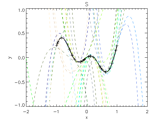

Fig.5a It's becoming messy!

Remark:

There is a couple of intrinsic IDL routines that do the cubic spline interpolation and smoothing. I didn't compare how does my routines compare in speed and accuracy.