But let's go step by step. Our task is to solve numerically the integral:
$$I = \int_a^b f(x)\, \mathrm{d} x.$$
The first step is to introduce a variable substitution $u$ that reduces the integration boundaries to the interval [-1, 1]:
$$x = \frac{b+a}{2} + \frac{b-a}{2} \, u.$$
It is clear that with this substitution the integration interval $[a, b]$ in $x$ translates in $[-1, 1]$ in $u$. Derivative of the substitution equation is:
$$\mathrm{d}x = \frac{b-a}{2} \, \mathrm{d}u$$. The integral then becomes:
$$I = \frac{b-a}{2} \int_{-1}^1 f\left(\frac{b+a}{2} + \frac{b-a}{2} \, u \right)\, \mathrm{d} u = \frac{b-a}{2} \int_{-1}^1 g(u)\, \mathrm{d} u.$$
The new function $g(u)$ can be expanded in Maclaurin series:
\begin{equation}g(u) = a_0 + a_1\,u + a_2\,u^2+...\end{equation}
The expansion can be substituted in the integral to get:
\begin{equation} \int_{-1}^1 g(u)\, \mathrm{d} u = \int_{-1}^1 (a_0 + a_1\,u + a_2\,u^2+...) \mathrm{d} u = 2\left(a_0 + \frac{a_2}{3} + \frac{a_4}{5} + ...\right).\end{equation}
Same is in other quadratures, we make an assumption that the unknown integral can be expressed as a discrete sum of the function values in a sample of arguments weighted with some optimal weights:
$$ \int_{-1}^1 g(u)\, \mathrm{d} u = \sum_{i=1}^n C_i\,g(u_i),$$
where $C_i$ and $u_i$ are unknown weights and discrete arguments. On the other hand, Maclaurin series converge for every $u \in [-1, 1]$, and thus for every point $u_i$ it holds:
$$g(u_i) = a_0 + a_1\,u_i + a_2\,u_i^2+...$$
If we use the last expression to write the discrete sum explicitly, we get:
\begin{eqnarray*}\sum_{i=1}^n C_i\,g(u_i) = C_1\,g(u_1) + ... + C_n\,g(u_n) &=& C_1\,( a_0 + a_1\,u_1 + a_2\,u_1^2+...) + \\ &+& C_2\,( a_0 + a_1\,u_2 + a_2\,u_2^2+...) + \\ &+&\,...\, +\\ &+& C_n\,( a_0 + a_1\,u_n + a_2\,u_n^2+...).\end{eqnarray*}
The right-hand side of the last equation must be equal to the right-hand side of Eq.2, thus we can write 2$n$ equations for 2$n$ unknowns ($C_i$ and $u_i$):
\begin{eqnarray*}a_0 &:& C_1 + ... + C_n = 2\\ a_1 &:& C_1u_1 + ... + C_n u_n = 0\\a_2 &:& C_1 u_1^2 + ... + C_n u_n^2 = 2/3\\ ... &:&... \\a_{2n-2} &:& C_1 u_1^{2n-2} + ... + C_n u_n^{2n-2} = 2/(2n-1)\\a_{2n-1} &:& C_1 u_1^{2n-1} + ... + C_n u_n^{2n-1} = 0.\end{eqnarray*}
This is a non-linear system with a non-trivial solution. However, Legendre found out that the values $u_i$ present zeros of the following polynomial:
\begin{equation}P_n(x) = \frac{1}{2^n n!}\frac{\mathrm{d}^n}{\mathrm{d}x^n}(x^2-1)^n\;\;\;(n = 0, 1, 2, ...)\end{equation}
This is the definition of the n-th order Legendre polynomial. These polynomials have several important characteristics:
(i) on the [-1, 1] interval, the n-th order polynomial has n real and unique zeros that are symmetrically distributed relative to $x = 0$;
(ii) $P_n(1) = 1$, for every $n$;
(iii) $P_n(-1) = (-1)^n$, for every $n$;
(iv) polynomial $P_{n+1}$ can be found from a recurrent formula:
$$(n+1)\, P_{n+1}(x) = (2n+1)\,x\,P_n(x) - n\,P_{n-1}(x).$$
Back to the initial task. Once the zeros $u_i$ and their weights $C_i$ are known, the integration is trivial.
IDL implementation
There are three steps that have to be solved:
(i) find the coefficients of Legendre polynomial of order $n$;
(ii) find the zeros of that polynomial;
(iii) find their weights.
The main IDL routine is legendre_polynomials.pro. It serves as a wrapper for the other three routines:
legendre_coefficients.pro - uses the recurrent formula to evaluate coefficients of Legendre polynomial for given $n$ (order);
legendre_zeros.pro - uses method of chords to find zeros of a Legendre polynomial specified by its coefficients;
legendre_weights.pro - solves a system of linear equations using Cramer's method to determine the weights of the zeros found in the previous step.
Note that the code is numerically accurate up to $n = 33$. The higher orders require higher precision. Anyway, $n = 33$ is more than enough in most of the common applications.
Example
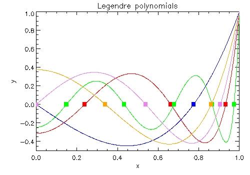
In the figure below I show Legendre polynomials on the $x\in[0, 1]$ interval (remember that they are symmetric in respect to $x=0$) for n = 3 (blue), n = 4 (orange), n = 5 (violet), n = 6 (red) and n = 10 (green). For each of them square-symbols show the zeros.
legendre_polynomials.tar - contains the IDL sav files described above,
legendre_zeros.tar - contains ASCII versions (just zeros and their weights).
Final remark
This program was originally written for the students of the practical part of the course "Analysis of astronomical observations" that I was teaching at the Faculty of mathematics in Belgrade. The course was initially shaped in the 70's by professor Dragutin Djurovic. His textbook "Mathematical analysis of astronomical observations" is a precious and rather unique manuscript that compiles many useful algorithms and methods from numerical mathematics, statistics and probability. The book describes the application of these methods to the realistic astronomical data. It remained rather unknown as it is written in Serbo-Croatian language and never reprinted.
Some weeks ago I heard sad news that professor Djurovic passed away at age 76. I had a chance to follow his course on my bachelor studies and later on to be his teaching assistant on the same course. I will remember him as a very particular character with a great sense of humor. His scientific papers (mainly in the field of solar activity and its influence on geophysical phenomena) as well as his aforementioned textbook remain as a proof that he was an excellent scientist, too.
No comments:
Post a Comment